Skip Navigation | ANU Home | Search ANU | Directories

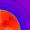
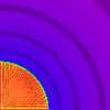
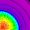
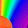
3D Noh Shock Test

This 3D test consists of a circular infinite strength shock propagating out from the origin on a square Cartesian grid. There are analytical solutions for 1D, 2D and 3D flows, ( see 1D Noh Test, 2D Noh Test).

The Noh shock, having an isothermal Mach number of 1000.0 in the tests, proves to the a difficult problem in 2D and 3D calculations. The well known striping or carbuncle instability increases in strength with the Mach number of the shock. If left unchecked the striping is very severe around a large portion of the expanding sphere (circle in 2D). This is almost certainly the reason for the failure of many codes in te Liska and Wendroff test paper to perform the 2D version of the test, especially with large CFL numbers. For example , of the successful codes, even PPM used a very small CFL = 0.2 for the LW 2D version of the test.

Here, and in the 2D Noh test, we apply the carbuncle/striping dissipation in the shock fronts and are able to obtain solutions, however the striping is so severe that it occurs even when there is significant curvature of the shock front w.r.t the grid, and applying to much smoothing affects the shock solution unacceptably. For practical purposes this restricts the code to Mach numbers less than 1000.0 for most shock geometries unless particular care is taken to modify the striping parameters for each individual case.

The 3D test here is for a cube 100x100x100 cells, to stress the resolution capabilities of the codes, and to have a test model that can be run with modest computing resources in a short time ( approx. 30 minutes on a single G5 processor ).

The 3D spherical inflow solution with Gamma = 5/3 is as follows:

The shock front expands at V_s = 1/3

Inside the shocked region: (r < t/3)

• Density = 64.0

• Pressure = 64/3

• Velocity = 0.0

Outside the shock: (r > t/3)

• Density = (1.0 + t/r)^2

• Pressure = 0.0

• Radial Velocity = -1.0

The code and configuration files for Fyris to run the 3D Noh problem will be available soon.

Initial Conditions:

• Adiabatic index: Gamma = 5/3

• Domain: 0.0 < x < 1.0, 0.0 < y < 1.0 , 1st quadrant.

• The density is uniform, d = 1.0 everywhere

• Pressure is set to P = 1.0e-6 everywhere, as an approximation to zero pressure.

• The radial velocity, v(r), is -1.0 (i.e. flowing towards the origin). This gives an isothermal Mach number, M_i = (v * d)/ P = 1000.0.

Ending Condition:

• Time, t = 2.0

Grid:

• 100 x 100 x 100 cells.

• Left, Bottom, and Yon boundaries are reflecting.

• Top, Right and Hither boundaries are updated each cycle with the analytical solution for the density, plus fixed inflow velocity and pressure - to allow the inflow to continue for an extended period of time.

Algorithm Settings:

• CFL number: 0.8

• Striping correction artificial viscosity parameter: alpha = 0.05

• DivV threshold: 1.0, Scale: 1.0 (standard)

• Flattening: minimum 0.0, maximum 1.0 (standard)

The code and configuration files plus output for Fyris to run the 3D Noh problem will be available here.

Results

L1 Norms w.r.t. Analytical model at t = 2.0

• L1 norm Density : 1.90 per cent

• L1 norm Pressure : 2.33 per cent

z = 0.0 plane
Final Density, z = 0.0 plane AutoMaxScale: ( 0, 66.957 )	Final Density, z = 0.5 plane AutoMaxScale: ( 0, 68.0824 )
Final Density, summed z planes AutoScale: ( 540.157, 4760.85 )	Pressure z = 0.5 plane AutoMaxScale: ( 0, 22.1986 )
Velocity_x, z = 0.5 plane AutoScale: ( -0.891715, 0.0610022 )	Velocity Magnitude, z = 0.5 plane AutoMaxScale: (0, 1.00175)
(min max)