Research School of Astronomy and Astrophysics
Fyris Alpha Simulation Code
|
Research School of Astronomy and Astrophysics
Fyris Alpha Simulation Code
|
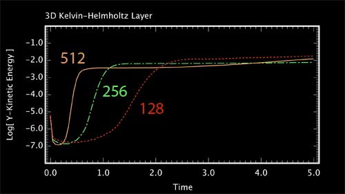
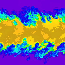
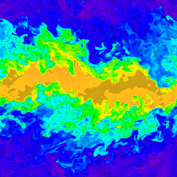
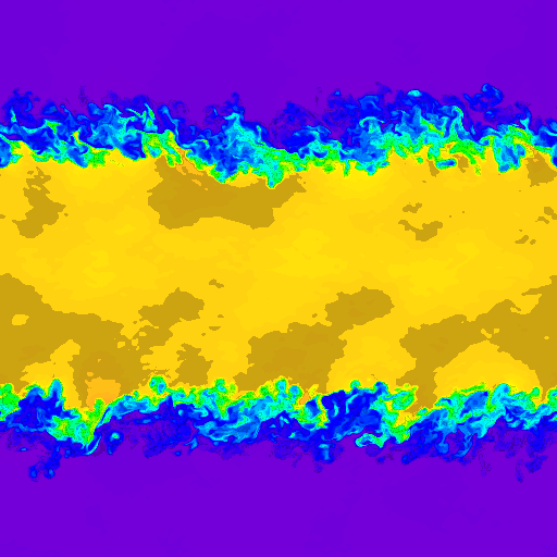
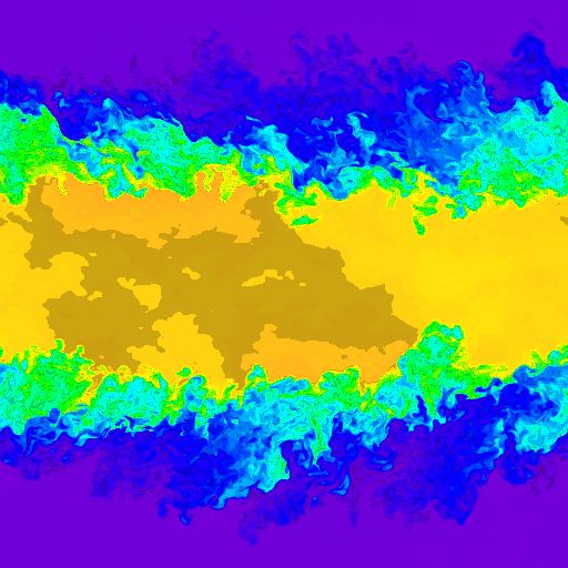
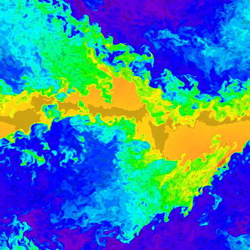
3D Kelvin–Helmholtz TestThis test consists of a dense central layer moving with respect to a lower density layer above and below the dense layer. Using periodiuc boundaries on all sides, a steady state can be established. Noise is added to the dense layer velocity field at the 1% level to seed the Kelvin-Helmholtz instability (KH instability). Note, the parameters here are identical to the 2D version of this problem, excepting only the presence of the third z-axis. There is not an analysitcal solution, but the growth of the y-component of the kinetic energy grows in essentially the same fashon as the test performed by the Athena code: (URL). There is a brief settling period, followed by exponential growth and finally saturation. The three resolutions excite increasing maximum wave number modes, and the higher wave number modes grow more quickly than the lower wave number modes, as expected. Initial Conditions:
Grid:
Algorithm Settings:
Ending Condition:
ResultsY-Axis Kinetic energy 0.5*d*v_y^2QuickTime Movies
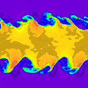
Central z = 0.0 Plane Images128 x 128 cells
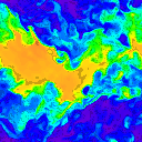
256 x 256 cells
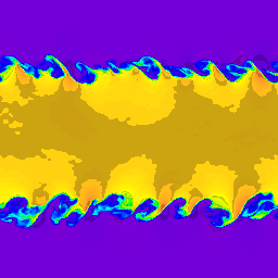
512 x 512 cells
|
|||||||||||||||||||||||||||||||
|
Page last updated: Wednesday, 19-May-2010 13:57:55 AEST Please direct all enquiries to: Ralph.Sutherland@anu.edu.au Page authorised by: Ralph Sutherland |
|
The Australian National University CRICOS Provider Number 00120C — ABN: 522 34063906 |