Skip Navigation | ANU Home | Search ANU | Directories

3D Constant Energy Bubble Test

This test models a constant energy wind bubble. The energy is injected as a spherically diverging supersonic wind, carrying most of the energy flux in the form of kinetic energy. There is a similarity solution for the radius as a power-law function of time. The bubble structure consists (from the centre outwards) of a free, supersonic, wind, terminated by a wind shock. Outside the wind shock is a high pressure region of shocked wind material, bounded by a contact discontinutity, r_c. Outside r_c, there is a dense layer of shocked ambient medium bounded by the outer shock, r_s.

Performing this model on a 3D Cartesian grid poses a series of challenges. The wind injection region is small compared to the overall gid domain, and in order to well sample the spherical flow to get a smooth wind and an accurate injection rate, quite high resolution is needed. In three dimensions, uniformly high resolution can be prohibitive, both in computation time and in memory requirements. Here the overall grid is defined with a resolution of 144x144x144 cells, and in order to get an accurate result, some form of refined mesh is needed. Currently Fyris Alpha supports predefined fixed refined embedded meshes, however it is hoped that this test can serve for fully adaptive approaches as well, either for other codes, and Fyris in future upgrades.

The radius of the bubble is expected to vary as r_s = k t^(3/5), when it achieves self-similarity. In order to start with a non-singular intial state, the wind injection region has a finite radius. This means that the bubble must evolve for sufficient time for r_s >> r_initial, so that the bubble can tend towards the self-similar powerlaw. This means the initial radius must be much smaller than the final bubble radius, which becomes difficult on a low resolution grid such as being used here.

In some cases deviations from perfect spherical symmetry occurs, mostly due to poor sampling of the inflow region, giving an uneven wind. To measure the effective radius of the bubbles in a robust way, we take the effective radius to be the cube root of the number of cells with speed greater than epsilon, times the cell width, dx.

r_eff = dx * (cells where |v| > epsilon)^(1/3),

where epsilon is chosen to be 1.0e-6. The ambient medium has an initial velocity of 0.0 everywhere, so this method accounts for all cells that have been overrun by the bubble and the wind.

Initial Conditions

Algorithm Settings

• Adiabatic Index = 5/3
• CFL number = 0.8
• Striping Control, viscosity alpha = 2.0e-3

Grid:

• Coarsest level, Cartesian 144x144x144 cells
• -1.0 < x < 1.0, -1.0 < y < 1.0, -1.0 < z < 0.0
• All boundaries are constant

It is up to the modeller if refined meshes are used, as long as the coarsest grid is 144^3, and the final radii are computed from the coarsest level.

Ambient medium:

• density = 1.0
• pressure = 0.01
• velocity = 0.0

Wind Boundary condition

• r_initial = r_wind = 0.02
• wind density = 0.1
• wind pressure = 0.1
• wind, radial velocity = 10.0

The region defined by r < r_wind is updated each cycle with the wind conditions. Note the origin can have a severe rarefaction problem at the origin, which does not evolve as the wind is refreshed each cycle, but the code needs to be able to cope with a single wind step.

This results in the boundary of the wind region advecting wind material onto the grid each cycle.

The boundary of the wind is not smoothed (and cannot be), however, the initial region in the ambient medium with r = 0.02 is partially evacuated to 0.001 of the orginal density and the edges of the resulting hole is smoothed with a gaussian FWHM = 1.0 cells, so that when the wind boudary region is imposed the flow in intially into a smoohed ambient medium surface.

Ending Condition

Time, t = 1.60

r_eff vs time fit interval, 1.0 < t < 1.6

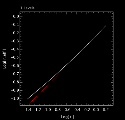
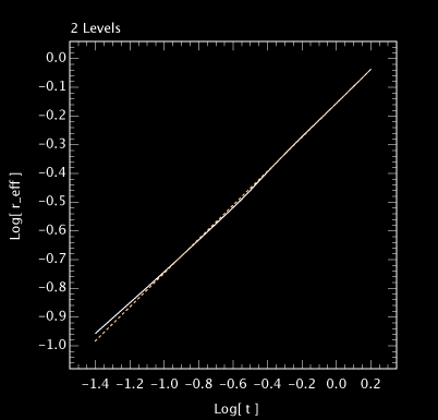
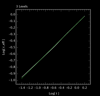
Results

Here 3 tests were run, a) single level uniform grid, b) a 2 level grid with a factor of 3 refinement over the central third of the grid domain, and c) a 3 level grid with factors of 3 refinement between each level, each successive level covering the central third of their super-levels. The effective resolution of model c is 1296^3 if it were computed as a single unform mesh. A 1296^3 cell grid would be slower by an estimated factor of approximately 504, than the three level 144^3 model. All were run on an 8cpu Sun v40z Opteron system with MPI.

1 Level

QuickTime Movies

Log Density, Central x-y plane (AutoScale)	Log Column Density (Auto Scale)	Log Pressure, Central x-y plane (AutoScale)
(min max)

2 Levels

QuickTime Movies

Log Density, Central x-y plane (AutoScale)	Log Column Density (Auto Scale)	Log Pressure, Central x-y plane (AutoScale)
(min max)

3 Levels

QuickTime Movies

Log Density, Central x-y plane (AutoScale)	Log Column Density (Auto Scale)	Log Pressure, Central x-y plane (AutoScale)
(min max)