|
|
AUSTRALIAN
NATIONAL UNIVERSITY Revision 1.00 Created: 5 December 2000 Last modified: 6 December 2000 |

NIFS USER'S MANUAL
Peter J. McGregor
Research School of Astronomy
and Astrophysics
Institute of Advanced
Studies
Australian National
University
Revision History
|
Revision No. |
Author & Date |
Approval & Date |
Description |
|
Revision 1 |
Peter J. McGregor 5 December 2000 |
|
Original document. |
|
|
|
|
|
Contents
5.3.2 AO Imaging
Spectropolarimetry
6.2 Configuring
the Science Instrument
6.2.1
Opening/Closing the Environmental Cover
6.2.2 Setting the
Focal Plane Mask Wheel
6.2.3 Setting the
Blocking Filter Wheel
6.2.4 Setting the
Grating Angle
6.3 Configuring
the Science Detector
6.3.1 Setting the
Read Out Method
6.3.2 Setting the
Integration Time
6.3.3 Setting the
Number of Fowler Samples
6.3.4 Setting the
NDR Read Out Period
6.3.5 Setting the
Number of Coadded Frames
6.3.6 Setting the
Number of Repeat Sequences
6.3.7 Configuring
the Quick Look Display
6.4 Configuring
the OIWFS Instrument
6.4.1 Initializing
and Setting the OIWFS X-Y Gimbal Mirror
6.4.2 Setting the
OIWFS Filter and Field Stop
6.5 Configuring
the OIWFS Detector
6.5.1 Setting the
Integration Time
6.5.2 Configuring
the Quick Look Display
6.6 Recording
Science Detector Bias Frames
6.7 Recording
Science Detector Dark Frames
6.8 Recording
Science Detector Dome Flats
6.9 Recording an
Arc Lamp Frame
6.10 Recording a
Spatial Calibration Frame
6.11 Locating the
Occulting Disks
6.12 Recording
OIWFS Detector Bias Frames
6.13 Recording
OIWFS Detector Dark Frames
6.14 Recording
OIWFS Detector Dome Flats
6.15 Calibrating
the OIWFS X-Y Gimbal Mirror
6.16 Recording
Science Detector Sky Flats
6.17 Recording
OIWFS Detector Sky Flats
6.20 Executing a
Science Observation
6.24 Checking
Science Detector Performance
6.25 Monitoring
Cryostat Temperatures
6.26 Initiating
the Rapid Warm-Up Sequence
7.1 Jets From
Young Stellar Objects
7.2 Massive Black
Holes in Nearby Galaxies
7.3 Inner
Narrow-Line Regions of Seyfert Galaxies
7.4 Imaging
Spectropolarimetry of Cygnus A
8.2 Forming BIAS
and DARK Frames
8.4 Defining the
Geometrical Calibration
8.5 Combining
Object and Sky Images
8.8 Interactively
Cleaning Bad Pixels
8.9 Applying the
Geometrical Transformation
8.13 Dividing by a
Smooth Spectrum Star
8.15 Plotting the
Final Spectra
8.16 Deriving
Polarization IQU Values
8.17 Plotting
Polarization Spectra
8.18 Plotting
Polarization Percentage and Position Angle Images
Appendix A: System
Performance
Appendix B:
Spectrophotometric Standards
Appendix C: Smooth
Spectrum Stars
Appendix D:
Near-Infrared Spectral Features of Astronomical Significance
Appendix E: Arc
Lamp Wavelengths
Appendix F: OH
Airglow Wavelengths
Appendix G:
Terrestrial Atmospheric Absorption
1 Purpose
This manual describes the operation of the Gemini Near-infrared Integral Field Spectrograph (NIFS) from a user’s point of view. It is the primary reference describing the instrument modes, how to prepare for an observing run, how to use the instrument effectively, and how to reduce data generated by the instrument.
2 Applicable Documents
|
Document ID |
Source |
Title |
|
|
|
|
3 Introduction
The Gemini Near-infrared Integral Field Spectrograph (NIFS) is the facility near-infrared spectrograph used with the ALTAIR adaptive optics system on Gemini North. NIFS is intended for near-diffraction limited imaging spectroscopy in the 0.94-2.5 mm wavelength range. As such, it is suitable for spectroscopic observations of complex high surface brightness structure, in a spatial or spectral sense, revealed at high spatial resolution by ALTAIR. NIFS records data at a two-pixel spectral resolving power of R ~ 5300. This moderate resolution is sufficient to significantly separate terrestrial OH emission lines. Post-detection OH suppression during data reduction significantly improves sensitivity relative to lower resolution instruments. The moderate spectral resolution is also suitable for dynamical studies of sufficiently high surface brightness astronomical objects.
4 Instrument Overview
This section will provide a general overview of the instrument and its observing modes; AO imaging spectroscopy, AO imaging spectropolarimetry, non-AO imaging spectroscopy, imaging spectroscopy using an occulting disk.
5 Preparing an Observation
5.1 Object Selection
This section will discuss issues that should be considered in selecting suitable objects for observation with NIFS; continuum surface brightness of structure on 0.1² spatial scales, emission-line surface brightness on 0.1² spatial scales, how to access on-line HST images to make these assessments, SNR expectations, saturation limits with and without the ND filter and occulting disks, spatial extent of the source and the need to mosaic, spectral features of interest between OH emission-line, sky subtraction versus dark subtraction strategies, sky determination from the image or via separate sky measurements by nodding the telescope, integration times to reduce the effect of dark current noise, precautions to avoid excessive detector remnance, position angle selection based on rectangular pixel size on the sky, the need to offset from a bright star to acquire very faint objects.
5.2 Guide Star Selection
This section will describe the guide star requirements for ALTAIR, the OIWFS, and the PWFS1 for both the natural guide star and laser guide star modes of ALTAIR. It will describe the operation of gs_search.pl and show how it should be used to identify suitable guide stars and determine their coordinates. It will also discuss likely zero point errors in various coordinate systems and make recommendations about ways of self-consistently defining PWFS1 guide star coordinates and science object coordinates.
5.3 Required Calibrations
5.3.1 AO Imaging Spectroscopy
This section will describe the calibration data that are required to extract scientific results from NIFS AO imaging spectroscopy data; bias frames, dark frames, flat field frames, a spatial calibration frame for correcting image distortion, smooth spectrum star spectra at the same airmass (±5%) for removing atmospheric absorption features, and spectrophotometric flux calibration star spectra. Many science programs will also need to determine the average PSF.
5.3.2 AO Imaging Spectropolarimetry
This section will describe the calibration data that are required to extract scientific results from NIFS AO imaging spectropolarimetry. These will generally be similar to §5.3.1 but will also include calibration of the waveplate polarizing efficiency and orientation (position angle zero point).
6 Operating the Instrument
6.1 Booting the System
This section will describe how to boot the system from a cold start. Visiting observers will not normally have to do this but it will be included for staff astronomers and for completeness.
6.2 Configuring the Science Instrument
This section will describe how to configure the mechanisms of the NIFS IFU spectrograph.
6.2.1 Opening/Closing the Environmental Cover
This section will describe how to operate the environmental cover – mainly as a reminder that this has to be done.
6.2.2 Setting the Focal Plane Mask Wheel
This section will describe how to set the Focal Plane Mask Wheel and will list its contents and the keywords used to identify them.
6.2.3 Setting the Blocking Filter Wheel
This section will describe how to set the Blocking Filter Wheel and will list its contents and the keywords used to identify them.
6.2.4 Setting the Grating Angle
This section will describe how to select the spectrograph grating to be used and how the grating angle can be varied over a small range to optimize the wavelength range recorded.
6.3 Configuring the Science Detector
This section will describe how to configure the NIFS IFU spectrograph detector and the associated Quick Look displays.
6.3.1 Setting the Read Out Method
This section will describe the read out methods of the NIFS science detector and how to select the active read out method. The read out methods offered will be Fowler sampling and linear fitting (integration up the ramp) . It will discuss the pros and cons of resetting the detector at the end of each integration; resetting the array avoids the saturation of bright sky emission lines, but it upsets the stability of the detector and may lead to unacceptably high dark current in subsequent frames.
6.3.2 Setting the Integration Time
This section will describe how to select and set the frame integration time for the NIFS science detector. It will discuss trade-offs between read noise (short integrations), dark current noise (long integrations), and variations in sky emission (on 5 min time scales).
6.3.3 Setting the Number of Fowler Samples
This section will discuss criteria for selecting and the method for setting the optimal number of Fowler samples to obtain at the beginning and end of integrations when using the Fowler sampling read out method. There is a trade-off here between the read noise reduction achieved and the extra dark current noise generated by accessing each pixel multiple times.
6.3.4 Setting the NDR Read Out Period
This section will discuss criteria for selecting and the method for setting the optimal Non-Destructive Read (NDR) period when using the linear fitting read out method. There is a trade-off here between the read noise reduction achieved and the extra dark current noise generated by accessing each pixel multiple times.
6.3.5 Setting the Number of Coadded Frames
This section will describe how to select and set the number of frames that are coadded before data are recorded to disk. Coadding frames is efficient when short integration times are used, but is not likely to be used on typical long integrations on science objects.
6.3.6 Setting the Number of Repeat Sequences
This section will describe how to select and set the number of repeat sequences. A sequence is defined as a basic data set; one set of coadded frames for imaging spectroscopy, but one full set of waveplate positions for imaging spectropolarimetry. Calibration data can usually be obtained more efficiently by recording multiple data sequences. Usually only one data sequence will be recorded on a science object before it is necessary to nod the telescope.
6.3.7 Configuring the Quick Look Display
This section will describe how to configure the science detector Quick Look Display to subtract a sky spectrum, extract and display a 1D spectrum, and display a 2D image over a specified wavelength range.
6.4 Configuring the OIWFS Instrument
This section will describe how to configure the mechanisms of the NIFS OIWFS.
6.4.1 Initializing and Setting the OIWFS X-Y Gimbal Mirror
This section will describe how to initialize the OIWFS X-Y gimbal mirror and how to set its so as to locate an OIWFS guide star.
6.4.2 Setting the OIWFS Filter and Field Stop
This section will describe how to set the OIWFS filter. The OIWFS filter should be set to the same pass band as the NIFS IFU spectrograph in order to minimize differential atmospheric refraction between the OIWFS and science instrument. The OIWFS filter wheel contains sets of identical filters, each with field stops of different diameters. The contents of the wheel will be listed and criteria for selecting the optimal field stop size for a particular application will be described.
6.5 Configuring the OIWFS Detector
This section will describe how to configure the NIFS OIWFS detector.
6.5.1 Setting the Integration Time
This section will describe how to select and set the frame integration time for the NIFS OIWFS detector. The OIWFS should be used for slow flexure compensation when tip-tilt and focus are being sensed by the ALTAIR AOWFS. Relatively long integrations on the OIWFS detector are possible in this mode. However, the OIWFS is used to sense rapid tip-tilt and focus changes when a laser guide star is used with the AOWFS. Integration times in the range 0.01-0.1 s are then required for the OIWFS detector.
6.5.2 Configuring the Quick Look Display
This section will describe how to configure the OIWFS detector Quick Look Display to subtract a sky spectrum and display the resulting image.
6.6 Recording Science Detector Bias Frames
This section will describe how to configure the instrument and record bias frames for the science detector.
6.7 Recording Science Detector Dark Frames
This section will describe how to configure the instrument and record dark frames for the science detector.
6.8 Recording Science Detector Dome Flats
This section will describe how to activate the GCAL flat field lamp, deploy the ISS science fold mirror to point to GCAL, configure the NIFS science instrument, configure the NIFS science detector, and record a sequence of lamp on/off flat field frames.
6.9 Recording an Arc Lamp Frame
This section will describe how to activate the GCAL arc lamp, deploy the ISS science fold mirror to point to GCAL, configure the NIFS science instrument, configure the NIFS science detector, and record a sequence of lamp on/off arc lamp frames for wavelength calibration.
6.10 Recording a Spatial Calibration Frame
This section will describe how to insert the Ronchi grid in the Focal Plane Mask Wheel and record a spatial calibration frame using the GCAL flat field lamp as the light source. This frame is used to determine and correct for image distortion.
6.11 Locating the Occulting Disks
This section will describe how to determine the pixel positions of the occulting disks in the Focal Plane Mask Wheel using the GCAL flat field lamp as the light source.
6.12 Recording OIWFS Detector Bias Frames
This section will describe how to configure the OIWFS and record bias frames for the OIWFS detector.
6.13 Recording OIWFS Detector Dark Frames
This section will describe how to configure the OIWFS and record dark frames for the OIWFS detector.
6.14 Recording OIWFS Detector Dome Flats
This section will describe how to activate the GCAL flat field lamp, deploy the ISS science fold mirror to point to GCAL, configure the NIFS OIWFS, configure the NIFS OIWFS detector, and record a sequence of lamp on/off flat field frames.
6.15 Calibrating the OIWFS X-Y Gimbal Mirror
This section will describe how to initialize the OIWFS X-Y gimbal mirror.
6.16 Recording Science Detector Sky Flats
This section will describe how to configure ALTAIR, deploy the ISS science fold mirror to point to ALTAIR, configure the NIFS science instrument, configure the NIFS science detector, and record a sequence of sky flats.
6.17 Recording OIWFS Detector Sky Flats
This section will describe how to configure ALTAIR, deploy the ISS science fold mirror to point to ALTAIR, configure the NIFS OIWFS, configure the NIFS OIWFS detector, and record a sequence of sky flats.
6.18 Acquiring an Object
This section will describe how to set the ISS rotator angle, acquire a PWFS1 guide star, begin active mirror correction, acquire an OIWFS star, begin tip-tilt and focus correction, view the science field with the telescope acquisition camera, record and display an undispersed object image using the NIFS flip mirror, center the object in the NIFS field using the Quick Look display, acquire the AOWFS star and begin adaptive correction, and spectrally-compress a dispersed NIFS image and display the sky image.
6.19 Focusing the Telescope
This section will describe how to fix the telescope focus that is maintained by the OIWFS.
6.20 Executing a Science Observation
This section will describe how to initiate a science observation and assess the result using the Quick Look Display.
6.21 Recording a PSF Star
This section will discuss considerations in recording a star spectrum with which to determine the PSF.
6.22 Interacting With ALTAIR
This section will describe what is needed to know about interacting with ALTAIR. It will describe how to deploy the ALTAIR feed mirror, set the ISS science fold mirror to point to ALTAIR, locate the AOWFS guide star, how to set the AOWFS integration time and servo-loop parameters, and how to define whether tip-tilt and focus control is derived from the AOWFS or from the OIWFS.
6.23 Interacting With GPOL
This section will describe what is needed to know about interacting with GPOL. It will describe how to insert GPOL into the beam, how to select which waveplate is used, how to select the K band wire grid in NIFS, and how to synchronize data taking with movement of the waveplate.
There are calibration issues here since the GCAL beam will not pass through GPOL or ALTAIR. These will be explained.
6.24 Interacting With GCAL
This section will describe what is needed to know about interacting with GCAL. This may be covered in the sections on recording flat field and wavelength calibration frames. However, there are general issues that need to be described, such as the fact that the GCAL beam does not pass through ALTAIR.
6.25 Checking Science Detector Performance
This section will describe how to record and analyze test data that quantifies the performance of the science detector. Typical ranges of the detector parameters will be listed so that users can determine whether or not the detector performance is optimal. Detector parameters that will be measured are read noise, dark current, remnance, quantum efficiency, and cross-talk. Users who find that the detector is operating outside the acceptable range will be encouraged to contact observatory staff.
6.26 Monitoring Cryostat Temperatures
This section will describe how to monitor the cryostat and detector temperatures and will list typical temperature ranges for these temperatures.
6.27 Initiating the Rapid Warm-Up Sequence
This section will describe how to initiate the rapid warm-up sequence. It will be cautioned that this should only be performed by qualified observatory staff.
6.28 Shutting Down the System
This section will describe how to shut down the system.
6.29 Archiving Your Data
This section will describe how visiting NIFS users can archive their data.
6.30 Summary of Commands
This section will contain a summary list of the commands used to control NIFS that can be used as a quick reference for experienced users.
7 Observing Scenarios
7.1 Jets From Young Stellar Objects
7.2 Massive Black Holes in Nearby Galaxies
7.3 Inner Narrow-Line Regions of Seyfert Galaxies
7.4 Imaging Spectropolarimetry of Cygnus A
8 Data Reduction Procedures
This section will describe the procedures used to reduce NIFS imaging spectroscopy data using IRAF.
8.1 Preparations
8.2 Forming BIAS and DARK Frames
8.2.1 BIAS Frames
8.2.2 DARK Frames
8.3 Linearity Correction
8.4 Defining the Geometrical Calibration
8.5 Combining Object and Sky Images
8.6 Flat Fielding
8.7 Fixing Known Bad Pixels
8.8 Interactively Cleaning Bad Pixels
8.9 Applying the Geometrical Transformation
8.10 Forming Data Cubes
8.11 Extracting 1D Spectra
8.12 Flux Calibration
8.13 Dividing by a Smooth Spectrum Star
8.14 Extracting a 2D Image
8.15 Plotting the Final Spectra
8.16 Deriving Polarization IQU Values
8.17 Plotting Polarization Spectra
8.18 Plotting Polarization Percentage and Position Angle Images
Appendix A: System Performance
This section will summarize NIFS system performance.
Appendix B: Spectrophotometric Standards
Suitable flux calibration stars are listed in Table 1. These stars are drawn from Carter & Meadows (1995, MNRAS, 276, 734), Persson et al. 1998 (AJ, 116, 2475), the UKIRT standards list, and Hunt et al. 1998 (AJ, 115,2594). Only stars brighter than K = 12 mag and bluer than J-K = 0.5 are selected.
Table 1: Spectrophotometric Standard Stars
|
Star |
RA (J2000) Dec |
SpT |
J |
H |
K |
Ref |
|
|
HD 590 |
00 10 16.82 |
-18 51 45.8 |
F2V |
9.195 |
8.969 |
8.947 |
1 |
|
FS 101 |
00 13 43.58 |
+30 37 59.9 |
… |
10.553 |
10.420 |
10.381 |
3 |
|
HR 9101 |
00 24 28.44 |
+07 49 00.2 |
… |
11.622 |
11.298 |
11.223 |
2 |
|
FS 2 |
00 55 09.93 |
+00 43 13.1 |
… |
10.707 |
10.509 |
10.467 |
3 |
|
AS 02-0 |
00 55 58.60 |
+39 10 09.0 |
… |
8.775 |
8.771 |
8.770 |
4 |
|
HR 9104 |
01 03 15.94 |
-04 20 49.1 |
… |
11.045 |
10.750 |
10.693 |
2 |
|
FS 104 |
01 04 59.43 |
+41 06 30.8 |
… |
10.534 |
10.437 |
10.406 |
3 |
|
HD 8864 |
01 27 29.57 |
+04 27 43.4 |
A5 |
8.631 |
8.510 |
8.474 |
1 |
|
FS 107 |
01 54 10.24 |
+45 50 37.7 |
… |
10.490 |
10.286 |
10.226 |
3 |
|
FS 4 |
01 54 37.72 |
+00 43 00.6 |
… |
10.547 |
10.318 |
10.279 |
3 |
|
HD 15189 |
02 26 26.32 |
-13 52 47.1 |
G0V |
8.460 |
8.159 |
8.126 |
1 |
|
HD 15274 |
02 27 45.52 |
+08 51 28.6 |
F5 |
8.490 |
8.276 |
8.250 |
1 |
|
HR 9105 |
02 33 32.26 |
+06 25 36.2 |
… |
11.309 |
10.975 |
10.897 |
2 |
|
AS 06-0 |
02 41 03.87 |
+47 41 22.9 |
… |
8.713 |
8.694 |
8.674 |
4 |
|
HD 17040 |
02 43 40.85 |
-17 28 53.3 |
F7V |
9.401 |
9.141 |
9.107 |
1 |
|
FS 7 |
02 57 21.17 |
+00 18 39.4 |
… |
11.102 |
10.981 |
10.942 |
3 |
|
FS 108 |
03 01 09.85 |
+46 58 47.7 |
… |
10.073 |
9.795 |
9.724 |
3 |
|
HD 18847 |
03 01 24.82 |
-19 59 13.7 |
F5V |
8.992 |
8.686 |
8.653 |
1 |
|
HR 9107 |
03 32 02.63 |
+37 20 38.8 |
… |
11.934 |
11.610 |
11.492 |
2 |
|
AS 08-0 |
03 38 08.19 |
+35 10 53.2 |
… |
8.744 |
8.723 |
8.697 |
4 |
|
HR 9108 |
03 41 02.26 |
+06 56 15.7 |
… |
11.737 |
11.431 |
11.337 |
2 |
|
FS 111 |
03 41 08.55 |
+33 09 35.5 |
… |
10.641 |
10.389 |
10.282 |
3 |
|
FS 112 |
03 47 40.70 |
-15 13 14.4 |
… |
11.203 |
10.950 |
10.893 |
3 |
|
AS 09-0 |
04 11 05.34 |
+60 10 24.7 |
… |
8.432 |
8.380 |
8.340 |
4 |
|
HD 29250 |
04 35 12.90 |
-29 38 09.8 |
A4IV |
9.465 |
9.361 |
9.354 |
1 |
|
FS 11 |
04 52 58.84 |
-00 14 41.5 |
… |
11.341 |
11.279 |
11.252 |
3 |
|
FS 119 |
05 02 57.44 |
-01 46 42.6 |
… |
9.916 |
9.873 |
9.850 |
3 |
|
AS 11-0 |
05 29 55.50 |
+39 38 59.0 |
… |
9.151 |
9.181 |
9.183 |
4 |
|
HD 37567 |
05 38 53.86 |
-12 46 33.3 |
B8/9V |
8.997 |
8.990 |
8.993 |
1 |
|
HR 9116 |
05 42 32.11 |
+00 09 02.2 |
… |
11.426 |
11.148 |
11.077 |
2 |
|
AS 12-1 |
05 52 21.51 |
+15 52 41.4 |
… |
11.241 |
10.931 |
10.866 |
4 |
|
HD 39944 |
05 54 43.18 |
-25 34 39.3 |
G1V |
8.465 |
8.144 |
8.104 |
1 |
|
FS 13 |
05 57 07.55 |
+00 01 11.1 |
… |
10.491 |
10.191 |
10.133 |
3 |
|
HD 40348 |
05 58 07.11 |
-02 33 27.9 |
A0 |
8.926 |
8.895 |
8.892 |
1 |
|
AS 14-0 |
06 11 24.80 |
+61 32 12.2 |
… |
8.688 |
8.623 |
8.590 |
4 |
|
AS 14-1 |
06 11 30.03 |
+61 32 04.7 |
… |
9.871 |
9.801 |
9.755 |
4 |
|
HR 9118 |
06 22 43.86 |
-00 36 28.9 |
… |
11.723 |
11.357 |
11.264 |
2 |
|
AS 15-0 |
06 40 34.31 |
+09 19 11.9 |
… |
10.874 |
10.669 |
10.628 |
4 |
|
HR 9122 |
07 00 51.79 |
+48 29 22.9 |
… |
11.680 |
11.408 |
11.356 |
2 |
|
AS 16-2 |
07 24 15.33 |
-00 32 47.7 |
… |
11.411 |
11.428 |
11.445 |
4 |
|
AS 16-4 |
07 24 17.56 |
-00 33 05.8 |
… |
11.402 |
11.106 |
11.043 |
4 |
|
HR 9126 |
07 30 34.49 |
+29 51 12.1 |
… |
11.876 |
11.522 |
11.450: |
2 |
|
HD 62388 |
07 43 15.04 |
-12 24 03.1 |
A0 |
8.727 |
8.691 |
8.670 |
1 |
|
HD 62998 |
07 46 07.66 |
-16 34 37.3 |
F6V |
8.593 |
8.323 |
8.294 |
1 |
|
HR 9131 |
08 25 42.99 |
+73 01 18.4 |
… |
10.819 |
10.546 |
10.499 |
2 |
|
HD 71264 |
08 26 18.18 |
-05 51 49.0 |
A0 |
8.612 |
8.565 |
8.538 |
1 |
|
HR 9134 |
08 29 25.10 |
+05 56 08.0 |
… |
11.881 |
11.624 |
11.575 |
2 |
|
HR 9135 |
08 36 12.61 |
-10 13 36.3 |
… |
12.362 |
12.098 |
12.040: |
2 |
|
AS 18-1 |
08 51 03.50 |
+11 45 03.0 |
… |
10.769 |
10.614 |
10.575 |
4 |
|
FS 123 |
08 51 11.78 |
+11 45 22.8 |
… |
10.173 |
10.185 |
10.212 |
3 |
|
AS 19-1 |
08 51 21.76 |
+11 52 37.7 |
… |
10.095 |
9.794 |
9.746 |
4 |
|
FS 18 |
08 53 35.42 |
-00 36 41.3 |
… |
10.812 |
10.570 |
10.521 |
3 |
|
FS 125 |
09 03 20.52 |
+34 21 02.9 |
… |
10.789 |
10.428 |
10.365 |
3 |
|
AS 20-0 |
09 19 27.66 |
+43 31 45.7 |
… |
9.551 |
9.519 |
9.497 |
4 |
|
HR 9138 |
09 41 35.91 |
+00 33 15.4 |
… |
11.354 |
11.041 |
10.981 |
2 |
|
HR 9139 |
09 42 58.33 |
+59 03 42.7 |
… |
11.683 |
11.338 |
11.276 |
2 |
|
HD 84503 |
09 45 08.58 |
-26 16 30.5 |
F2V |
8.849 |
8.638 |
8.579 |
1 |
|
HR 9141 |
09 48 56.40 |
-10 30 32.0 |
… |
11.081 |
10.775 |
10.715 |
2 |
|
HR 9142 |
10 06 28.88 |
+41 01 24.9 |
… |
11.993 |
11.729 |
11.686 |
2 |
|
HD 88449 |
10 11 40.38 |
-15 25 25.4 |
F5V |
8.522 |
8.257 |
8.223 |
1 |
|
AS 21-0 |
10 28 42.10 |
+36 46 18.0 |
… |
9.061 |
9.043 |
9.031 |
4 |
|
HR 9143 |
10 33 51.66 |
+04 49 04.6 |
… |
12.344 |
12.121 |
12.067 |
2 |
|
HD 94949 |
10 57 49.22 |
+09 01 07.4 |
F8 |
8.267 |
7.968 |
7.938 |
1 |
|
HD 100501 |
11 33 48.19 |
-29 21 39.3 |
A9V |
9.305 |
9.119 |
9.087 |
1 |
|
AS 23-0 |
12 02 53.41 |
+04 08 45.9 |
… |
8.889 |
8.847 |
8.828 |
4 |
|
HR 9145 |
12 13 12.00 |
+64 28 56.0 |
… |
11.958 |
11.711 |
11.664 |
2 |
|
HR 9148 |
12 14 25.40 |
+35 35 55.0 |
… |
11.642 |
11.378 |
11.324 |
2 |
|
HD 106973 |
12 18 09.33 |
-01 10 01.6 |
F8 |
9.148 |
8.875 |
8.836 |
1 |
|
HR 9149 |
12 21 39.27 |
-00 07 12.1 |
… |
12.213 |
11.917 |
11.861 |
2 |
|
AS 24-0 |
12 35 15.47 |
+62 56 56.4 |
… |
9.398 |
9.345 |
9.338 |
4 |
|
FS 133 |
13 15 52.53 |
+46 06 38.1 |
… |
12.292 |
11.940 |
11.868 |
3 |
|
HR 9150 |
13 17 29.31 |
-05 32 38.1 |
… |
11.661 |
11.310 |
11.250 |
2 |
|
HR 9152 |
13 58 40.22 |
+52 06 25.9 |
… |
11.149 |
10.878 |
10.831 |
2 |
|
HR 9153 |
14 07 33.76 |
+12 23 50.7 |
… |
11.947 |
11.605 |
11.560 |
2 |
|
AS 27-0 |
14 40 06.96 |
+00 01 45.4 |
… |
10.910 |
10.781 |
10.761 |
4 |
|
HR 9155 |
14 40 57.96 |
-00 27 45.8 |
… |
12.045 |
11.701 |
11.622 |
2 |
|
HD 129540 |
14 43 13.81 |
-02 57 31.1 |
A2V |
8.466 |
8.283 |
8.247 |
1 |
|
HR 9156 |
14 51 58.28 |
+71 43 16.4 |
… |
10.873 |
10.588 |
10.523 |
2 |
|
HR 9158 |
14 58 33.18 |
+37 08 31.9 |
… |
11.640 |
11.277 |
11.210 |
2 |
|
AS 28-0 |
15 09 20.30 |
+39 25 49.0 |
… |
8.455 |
8.378 |
8.372 |
4 |
|
AS 29-0 |
15 38 33.41 |
+00 14 17.9 |
… |
10.234 |
9.842 |
9.760 |
4 |
|
HR 9160 |
15 39 04.17 |
+00 15 01.9 |
… |
10.914 |
10.701 |
10.649 |
2 |
|
HR 9162 |
15 59 13.65 |
+47 36 42.5 |
… |
12.258 |
11.924 |
11.856 |
2 |
|
HD 147778 |
16 24 26.00 |
-17 44 42.0 |
F0V |
8.453 |
8.151 |
8.088 |
1 |
|
HR 9164 |
16 26 42.86 |
+05 52 23.4 |
… |
12.180 |
11.895 |
11.842 |
2 |
|
HD 148332 |
16 27 23.37 |
-01 22 27.4 |
F5 |
8.480 |
8.218 |
8.174 |
1 |
|
FS 138 |
16 28 06.72 |
+34 58 48.3 |
… |
10.442 |
10.413 |
10.411 |
3 |
|
HR 9166 |
16 31 33.76 |
+30 08 46.9 |
… |
11.816 |
11.479 |
11.419 |
2 |
|
HD 149226 |
16 33 28.44 |
-03 32 04.8 |
A5 |
8.006 |
7.667 |
7.588 |
1 |
|
HD 154066 |
17 03 46.49 |
-12 51 44.9 |
B8V |
7.962 |
7.845 |
7.812 |
1 |
|
HR 9169 |
17 13 44.86 |
+54 33 18.3 |
… |
11.355 |
11.118 |
11.075 |
2 |
|
FS 140 |
17 13 22.65 |
-18 53 33.8 |
… |
10.786 |
10.432 |
10.360 |
3 |
|
HR 9170 |
17 27 22.26 |
-00 19 24.6 |
… |
11.132 |
10.835 |
10.739 |
2 |
|
AS 31-0 |
17 44 06.76 |
-00 24 57.6 |
… |
10.744 |
10.644 |
10.602 |
4 |
|
HD 161961 |
17 48 36.86 |
-02 11 46.4 |
B0.5III |
7.369 |
7.330 |
7.323 |
1 |
|
FS 141 |
17 48 59.05 |
+23 17 43.4 |
… |
11.170 |
10.879 |
10.805 |
3 |
|
HD 166733 |
18 12 08.33 |
-02 15 29.4 |
F8 |
8.495 |
8.190 |
8.130 |
1 |
|
FS 35 |
18 27 13.48 |
+04 03 09.8 |
… |
12.194 |
11.840 |
11.739 |
3 |
|
AS 32-0 |
18 36 10.5 |
+65 04 30.0 |
… |
8.017 |
7.917 |
7.925 |
4 |
|
HR 9177 |
18 39 33.87 |
+49 05 37.6 |
… |
12.104 |
11.764 |
11.688 |
2 |
|
FS 147 |
19 01 55.27 |
+42 29 19.6 |
… |
9.910 |
9.883 |
9.865 |
3 |
|
HR 9178 |
19 01 55.40 |
-04 29 12.0 |
… |
10.966 |
10.658 |
10.566 |
2 |
|
AS 34-0 |
19 17 34.59 |
+48 06 03.2 |
… |
8.443 |
8.434 |
8.436 |
4 |
|
FS 148 |
19 41 23.43 |
-03 50 57.2 |
… |
9.509 |
9.490 |
9.477 |
3 |
|
FS 149 |
20 00 39.15 |
+29 58 37.4 |
… |
10.104 |
10.082 |
10.086 |
3 |
|
HD 193727 |
20 22 15.40 |
-16 06 49.0 |
F0V |
8.977 |
8.826 |
8.783 |
1 |
|
AS 35-0 |
20 35 11.20 |
+36 08 49.0 |
… |
8.625 |
8.544 |
8.524 |
4 |
|
FS 150 |
20 36 08.40 |
+49 38 24.4 |
… |
10.157 |
10.009 |
9.956 |
3 |
|
HR 9182 |
20 41 05.42 |
-05 03 42.6 |
… |
11.479 |
11.142 |
11.082 |
2 |
|
HR 9183 |
20 52 47.41 |
+06 40 03.9 |
… |
12.247 |
11.940 |
11.873 |
2 |
|
HD 201916 |
21 12 35.11 |
+00 53 36.2 |
F0 |
7.999 |
7.819 |
7.786 |
1 |
|
FS 151 |
21 04 14.82 |
+30 30 21.6 |
… |
12.206 |
11.943 |
11.869 |
3 |
|
HR 9185 |
22 02 05.66 |
-01 06 01.6 |
… |
12.021 |
11.662 |
11.586 |
2 |
|
HD 210427 |
22 10 51.36 |
-26 54 03.2 |
G1V |
9.245 |
8.895 |
8.852 |
1 |
|
HD 210863 |
22 13 26.42 |
-08 13 46.4 |
G0 |
8.590 |
8.272 |
8.234 |
1 |
|
AS 37-0 |
22 25 20.70 |
+40 09 38.0 |
… |
8.669 |
8.678 |
8.635 |
4 |
|
HD 212874 |
22 27 19.52 |
+04 02 50.4 |
A2 |
9.077 |
8.921 |
8.890 |
1 |
|
HD 214497 |
22 38 44.91 |
-14 48 46.7 |
F6V |
9.237 |
8.951 |
8.906 |
1 |
|
AS 38-2 |
22 41 50.20 |
+01 12 43.0 |
… |
11.355 |
11.026 |
10.991 |
|
|
HR 9186 |
23 18 10.00 |
+00 32 56.0 |
… |
11.403 |
11.120 |
11.045 |
2 |
|
HR 9187 |
23 23 34.27 |
-15 21 09.2 |
… |
11.857 |
11.596 |
11.538 |
2 |
|
HR 9188 |
23 30 33.22 |
+38 18 56.7 |
… |
11.634 |
11.337 |
11.257 |
2 |
|
HD 221462 |
23 32 27.40 |
-24 55 57.3 |
G3V |
8.630 |
8.282 |
8.219 |
1 |
|
AS 40-5 |
23 58 43.23 |
+61 09 40.2 |
… |
9.488 |
9.418 |
9.405 |
4 |
|
|
|
|
|
|
|
|
|
|
|
|
|
|
|
|
|
|
|
|
|
|
|
|
|
|
|
|
|
|
|
|
|
|
|
|
|
|
|
|
|
|
|
|
|
|
|
|
|
|
|
|
|
|
|
|
|
|
|
|
|
|
|
|
|
|
|
|
|
|
|
|
|
|
|
|
|
|
|
|
|
|
|
|
|
|
|
|
|
|
|
|
|
|
|
|
|
|
|
|
|
|
|
|
|
|
|
|
|
|
|
|
|
|
|
|
|
|
|
|
|
|
|
|
|
|
|
|
|
|
|
|
|
|
|
|
|
|
|
|
|
|
|
|
|
|
|
|
|
|
|
|
|
|
|
|
|
|
|
|
|
|
Appendix C: Smooth Spectrum Stars
This section will list suitable smooth spectrum stars.
Appendix D: Unpolarized Standards
The unpolarized stars below are taken from “Planets, Stars, & Nebulae Studied With Photopolarimetry”, 1974, T. Gehrels (ed.), University of Arizona Press, Tucson, 168 (via the UKIRT web pages). Most unpolarized stars have large proper motions. If the stars in this list are not appropriate then it is probably acceptable to use other stars with large proper motions.
Table 2: Unpolarized Standard Stars
|
Star |
RA (J2000) Dec |
ma |
md |
SpT |
K (mag) |
|
|
|
0 |
|
|
|
|
… |
|
|
0 |
|
|
|
|
… |
Appendix E: Polarized Standards
Polarized standards are polarized by dichroic absorption in the interstellar (or intracloud) medium). The “Serkowski” polarized standards in Table 3 are taken from “Planets, Stars, & Nebulae Studied With Photopolarimetry”, 1974, T. Gehrels (ed.), University of Arizona Press, Tucson, 170 (via the UKIRT web pages). They are based on fitting the Serkowski interstellar polarization law:
![]()
The maximum polarization, Pmax, occurs at the wavelength lmax.
Table 3: “Serkowski” Polarized Standard Stars
|
Star |
RA (J2000) Dec |
SpT |
Pmax (%) |
lmax (mm) |
P.A. (deg) |
K (mag) |
|
|
HD 23512 |
0 |
|
… |
2.3 |
0.60 |
30 |
… |
|
HD 204827 |
0 |
|
… |
5.6 |
0.46 |
60 |
… |
The fainter polarized stars in r Oph (Table 4) are taken from Sato et al. (1988, MNRAS, 230, 321). These still need to be checked for suitable guide stars.
Table 4: Polarized Embedded Stars
|
Star |
RA (J2000) Dec |
PK (%) |
s(PK) (%) |
P.A. (deg) |
K (mag) |
|
|
WL 1 |
0 |
|
3.51 |
0.54 |
157 |
10.58 |
|
WL 2 |
0 |
|
3.29 |
0.61 |
35 |
10.78 |
|
WL 3 |
|
|
2.17 |
0.68 |
126 |
11.07 |
|
WL 4 |
|
|
2.13 |
0.17 |
177 |
9.17 |
|
WL 5 |
|
|
5.88 |
0.44 |
153 |
10.12 |
|
WL 6 |
|
|
5.05 |
0.66 |
130 |
10.06 |
|
WL 7 |
|
|
1.40 |
0.50 |
170 |
11.04 |
|
WL 8 |
|
|
5.60 |
0.60 |
168 |
9.46 |
|
WL 9 |
|
|
3.82 |
1.07 |
28 |
11.80 |
|
WL 10 |
|
|
3.07 |
0.41 |
55 |
8.78 |
|
WL 12 |
|
|
4.90 |
0.23 |
50 |
8.99 |
|
WL 13 |
|
|
1.54 |
0.20 |
93 |
9.19 |
|
WL 14 |
|
|
2.16 |
0.94 |
54 |
11.69 |
|
WL 15 |
|
|
6.52 |
0.07 |
22 |
7.04 |
|
WL 16 |
|
|
4.87 |
0.23 |
27 |
7.81 |
|
WL 17 |
|
|
4.99 |
0.41 |
42 |
10.14 |
|
WL 18 |
|
|
1.14 |
0.26 |
45 |
9.85 |
|
WL 19 |
|
|
7.41 |
0.67 |
46 |
10.89 |
|
WL 20 |
|
|
5.21 |
0.35 |
56 |
9.11 |
|
GS 26 |
|
|
4.04 |
0.14 |
171 |
9.34 |
|
VS 5 |
|
|
3.13 |
0.20 |
19 |
9.99 |
|
VS 18 |
|
|
0.68 |
0.15 |
164 |
9.49 |
Appendix F: Near-Infrared Spectral Features of Astronomical Significance
Near-infrared spectral features that have been detected in astronomical objects are listed in Table 5.
Table 5: Vacuum(?) Wavelengths of Spectral Features of Astronomical Significance
|
Wavelength (mm) |
Identification |
Wavelength (mm) |
Identification |
|
0.991272 |
[S VIII] 2p5 2P03/2-2P01/2 |
1.572 |
He II 13-7 |
|
0.999756 |
Fe II |
1.58 |
12CO 4-1 |
|
1.00494 |
H I Pd |
1.58805 |
H I Br14 |
|
1.01236 |
He I |
1.59 |
Si I |
|
1.0174 |
Fe II |
1.599 |
[Fe II] |
|
1.03998 |
[N I] |
1.60 |
12CO 5-2 |
|
1.0300 |
[S II] |
1.6022 |
H2 6-4 Q(1) |
|
1.0490 |
Fe II |
1.607 |
[Si I] |
|
1.0501 |
Fe II |
1.61093 |
H I Br13 |
|
1.0747 |
[Fe XIII] |
1.6131 |
H2 5-3 O(3) |
|
1.0798 |
[Fe XIII] |
1.62 |
12CO 6-3 |
|
1.082909 |
He I |
1.64 |
12CO 7-4 |
|
1.083025 |
He I 23P-23S |
1.64072 |
H I Br12 |
|
1.083034 |
He I |
1.6435 |
[Fe II] a4D7/2-a4F9/2 |
|
1.0863 |
Fe II |
1.6454 |
[Si I] |
|
1.09381 |
H I Pg |
1.66 |
12CO 8-5 |
|
1.11126 |
Fe II |
1.664 |
[Fe II] |
|
1.1287 |
O I |
1.677 |
[Fe II] a4F7/2-a4D1/2 |
|
1.16264 |
He I |
1.68065 |
H I Br11 |
|
1.1883 |
[P II] |
1.688 |
Fe II |
|
1.1910 |
[Ni II] |
1.692 |
He II 12-7 |
|
1.233 |
H2 3-1 S(1) |
1.700247 |
He I 43D-33P |
|
1.25235 |
[S IX] 329 eV |
1.736 |
C IV 9-8 |
|
1.2521 |
[Fe II] a6D3/2-a4D1/2 |
1.73621 |
H I Br10 |
|
1.2527 |
He I 33S-43P0 |
1.77 |
C2 |
|
1.2567 |
[Fe II] a6D1-a4d7 |
1.81741 |
H I Br9 |
|
1.270 |
[Fe II] |
1.8358 |
H2 1-0 S(5) |
|
1.28181 |
H I Pb |
1.87510 |
H I Pa |
|
1.294 |
[Fe II] |
1.94456 |
H I Br8 |
|
1.298 |
[Fe II] |
1.9499 |
H2 2-1 S(5) |
|
1.313 |
H2 4-2 S(1), 3-1 Q(1,2,3) |
1.9576 |
H2 1-0 S(3) |
|
1.3164 |
O I |
1.96287 |
[Si VI] 2p5 2P03/2-2P01/2 |
|
1.321 |
[Fe II] |
1.99 |
Ca I |
|
1.4305 |
[Si X] |
2.0041 |
H2 2-1 S(4) |
|
1.476 |
He II 9-6 |
2.0338 |
H2 1-0 S(2) |
|
1.502499 |
Mg I 3S-3P0 |
2.040 |
[Al IX] |
|
1.504024 |
Mg I 3S-3P0 |
2.047 |
[Fe II] a4P-a2P |
|
1.504770 |
Mg I 3S-3P0 |
2.058130 |
He I 21P-21S |
|
1.51918 |
H I Br20 |
2.061 |
Fe II c4F-z4F0 |
|
1.522 |
[Fe II] |
2.0735 |
H2 2-1 S(3) |
|
1.52606 |
H I Br19 |
2.089 |
Fe II c4F3/2-z4F03/2 |
|
1.533 |
[Fe II] |
2.112007 |
He I 43S-33P |
|
1.53418 |
H I Br18 |
2.112143 |
He I |
|
1.54389 |
H I Br17 |
2.113203 |
He I 41S-31P |
|
1.55565 |
H I Br16 |
2.1218 |
H2 1-0 S(1) |
|
1.56 |
12CO 3-0 |
2.137 |
Mg II 5p2P3/2-5s2S1/2 |
|
1.57007 |
H I Br15 |
2.144 |
Mg II 5p2P1/2-5s2S1/2 |
|
2.1451 |
[Fe III] 3G3-3H4 |
|
|
|
2.1542 |
H2 2-1 S(2) |
|
|
|
2.16553 |
H I Brg |
|
|
|
2.189 |
He II 7-10 |
|
|
|
2.205644 |
Na I 42S-42P0 |
|
|
|
2.208367 |
Na I 42S-42P0 |
|
|
|
2.2178 |
[Fe III] 3G5-3H6 |
|
|
|
2.2233 |
H2 1-0 S(0) |
|
|
|
2.2420 |
[Fe III] 3G4-3H4 |
|
|
|
2.2477 |
H2 2-1 S(1) |
|
|
|
2.26 |
Ca I |
|
|
|
2.295 |
12CO 2-0 |
|
|
|
2.32141 |
[Ca VIII] 3p 2P01/2-2P03/2 |
|
|
|
2.324 |
12CO 3-1 |
|
|
|
2.334841 |
Na I |
|
|
|
2.337913 |
Na I |
|
|
|
2.345 |
13CO 2-0 |
|
|
|
2.3479 |
[Fe III] 3G5-3H5 |
|
|
|
2.354 |
12CO 4-2 |
|
|
|
2.3556 |
H2 2-1 S(0) |
|
|
|
2.374 |
13CO 3-1 |
|
|
|
2.385 |
12CO 5-3 |
|
|
|
2.3865 |
H2 3-2 S(1) |
|
|
|
2.404 |
13CO 4-2 |
|
|
|
2.4066 |
H2 1-0 Q(1) |
|
|
|
2.4134 |
H2 1-0 Q(2) |
|
|
|
2.414 |
12CO 6-4 |
|
|
|
2.42 |
C IV 10-9 |
|
|
|
2.4237 |
H2 1-0 Q(3) |
|
|
|
2.434 |
13CO 5-3 |
|
|
|
2.4375 |
H2 1-0 Q(4) |
|
|
|
2.446 |
12CO 7-5 |
|
|
|
2.4547 |
H2 1-0 Q(5) |
|
|
|
2.465 |
13CO 6-4 |
|
|
|
2.4754 |
H2 1-0 Q(6) |
|
|
|
2.479 |
12CO 8-6 |
|
|
|
2.48266 |
[Si VII] 2p4 3P2-3P1 |
|
|
|
|
|
|
|
|
|
|
|
|
|
|
|
|
|
|
|
|
|
|
|
|
|
|
|
|
|
|
|
|
|
|
|
|
|
|
|
|
|
|
|
|
|
|
|
|
|
|
|
|
|
|
|
|
|
|
|
|
|
|
|
|
|
|
|
|
|
|
|
|
|
|
|
|
|
Appendix G: Arc Lamp Wavelengths
This section will list the wavelengths of near-infrared emission lines in the GCAL arc lamps and plot spectra for each NIFS grating. The spectra below were recorded at a resolving power of ~ 1000 with PIFS on the Palomar 200 inch telescope and are taken from the PIFS web page. Line lists are tabulated.
Table 6: Air Wavelengths and Relative Intensities for Neon
|
Wavelength (mm) |
Relative Intensity |
Wavelength (mm) |
Relative Intensity |
|
1.11430 |
30 |
2.24281 |
4 |
|
1.11775 |
35 |
2.24668 |
1 |
|
1.13904 |
16 |
2.25304 |
23 |
|
1.14091 |
11 |
2.26618 |
4 |
|
1.15227 |
30 |
2.31005 |
6 |
|
1.15250 |
15 |
2.32603 |
10 |
|
1.15363 |
10 |
2.33730 |
11 |
|
1.16015 |
5 |
2.35654 |
9 |
|
1.16141 |
12 |
2.36365 |
35 |
|
1.16880 |
3 |
2.37016 |
3 |
|
1.17668 |
20 |
2.37076 |
11 |
|
1.17890 |
15 |
2.37092 |
11 |
|
1.17899 |
5 |
2.39514 |
18 |
|
1.19849 |
10 |
2.39565 |
6 |
|
1.20663 |
30 |
2.39781 |
10 |
|
1.24594 |
8 |
2.40985 |
2 |
|
1.25950 |
3 |
2.41614 |
5 |
|
1.26892 |
10 |
2.42696 |
6 |
|
1.27695 |
3 |
2.43650 |
15 |
|
1.29120 |
11 |
2.43716 |
8 |
|
1.32192 |
7 |
2.43834 |
1 |
|
1.49849 |
1 |
2.44479 |
4 |
|
1.49863 |
1 |
2.44594 |
7 |
|
1.52307 |
8 |
2.44597 |
7 |
|
1.54076 |
1 |
2.47765 |
4 |
|
1.54091 |
1 |
2.49037 |
2 |
|
1.71619 |
4 |
2.49289 |
5 |
|
1.71817 |
2 |
|
|
|
1.71825 |
2 |
|
|
|
1.71843 |
2 |
|
|
|
1.80832 |
1 |
|
|
|
1.82767 |
3 |
|
|
|
1.82826 |
2 |
|
|
|
1.83040 |
1 |
|
|
|
1.83849 |
1 |
|
|
|
1.83900 |
2 |
|
|
|
1.84029 |
1 |
|
|
|
1.84224 |
1 |
|
|
|
1.85915 |
1 |
|
|
|
1.85977 |
2 |
|
|
|
1.95771 |
2 |
|
|
|
2.03502 |
1 |
|
|
|
2.10413 |
12 |
|
|
|
2.17081 |
8 |
|
|
|
2.22473 |
3 |
|
|
Table 7: Vacuum Wavelengths and Relative Intensities for Argon
|
Wavelength (mm) |
Relative Intensity |
Wavelength (mm) |
Relative Intensity |
|
1.10819 |
10 |
1.40975 |
150 |
|
1.11095 |
3 |
1.42531 |
8 |
|
1.13968 |
8 |
1.42608 |
13 |
|
1.14450 |
12 |
1.45997 |
11 |
|
1.14707 |
6 |
1.46384 |
30 |
|
1.14912 |
120 |
1.46543 |
30 |
|
1.15835 |
1 |
1.46974 |
4 |
|
1.16719 |
200 |
1.47432 |
5 |
|
1.16908 |
1 |
1.50506 |
100 |
|
1.17227 |
10 |
1.51768 |
25 |
|
1.17364 |
9 |
1.53061 |
40 |
|
1.18877 |
4 |
1.53335 |
9 |
|
1.18999 |
1 |
1.53530 |
7 |
|
1.19466 |
12 |
1.53573 |
3 |
|
1.20299 |
2 |
1.54068 |
6 |
|
1.21156 |
150 |
1.59040 |
10 |
|
1.21430 |
30 |
1.59939 |
25 |
|
1.21547 |
2 |
1.61271 |
1 |
|
1.23468 |
30 |
1.61844 |
4 |
|
1.23597 |
10 |
1.64411 |
13 |
|
1.24062 |
100 |
1.65244 |
30 |
|
1.24427 |
300 |
1.65538 |
8 |
|
1.24595 |
100 |
1.67446 |
9 |
|
1.24911 |
200 |
1.69452 |
500 |
|
1.25577 |
2 |
1.74497 |
11 |
|
1.26251 |
2 |
1.78289 |
5 |
|
1.27369 |
30 |
1.79196 |
40 |
|
1.27497 |
12 |
1.84232 |
2 |
|
1.28062 |
200 |
1.84328 |
10 |
|
1.29602 |
500 |
1.98229 |
5 |
|
1.30118 |
200 |
1.99712 |
4 |
|
1.30320 |
2 |
2.03226 |
2 |
|
1.32176 |
200 |
2.06219 |
50 |
|
1.32317 |
200 |
2.06528 |
2 |
|
1.32345 |
200 |
2.07393 |
2 |
|
1.32763 |
500 |
2.08167 |
2 |
|
1.33059 |
4 |
2.09918 |
30 |
|
1.33168 |
800 |
2.13387 |
1 |
|
1.33338 |
6 |
2.15401 |
8 |
|
1.33708 |
1000 |
2.20456 |
1 |
|
1.34102 |
100 |
2.20832 |
8 |
|
1.35031 |
30 |
2.31395 |
20 |
|
1.35079 |
1000 |
2.38515 |
1 |
|
1.35479 |
8 |
2.39731 |
20 |
|
1.35773 |
12 |
2.51321 |
25 |
|
1.36030 |
40 |
|
|
|
1.36264 |
400 |
|
|
|
1.36823 |
200 |
|
|
|
1.37223 |
1000 |
|
|
|
1.38321 |
9 |
|
|
|
1.39113 |
8 |
|
|
|
1.39144 |
50 |
|
|
Table 8: Vacuum Wavelengths and Relative Intensities for Krypton
|
Wavelength (mm) |
Relative Intensity |
Wavelength (mm) |
Relative Intensity |
|
1.08779 |
80 |
1.58951 |
100 |
|
1.11902 |
100 |
1.63196 |
50 |
|
1.12608 |
200 |
1.64703 |
70 |
|
1.12622 |
150 |
1.65775 |
70 |
|
1.14606 |
500 |
1.67311 |
200 |
|
1.17956 |
150 |
1.67897 |
2000 |
|
1.18226 |
1500 |
1.68581 |
1000 |
|
1.20004 |
600 |
1.68951 |
2400 |
|
1.20805 |
160 |
1.69404 |
1800 |
|
1.21211 |
140 |
1.70746 |
40 |
|
1.21268 |
40 |
1.71034 |
600 |
|
1.22079 |
800 |
1.72354 |
30 |
|
1.27859 |
150 |
1.73724 |
700 |
|
1.28019 |
120 |
1.74092 |
120 |
|
1.28654 |
100 |
1.76216 |
150 |
|
1.28824 |
750 |
1.78476 |
650 |
|
1.29888 |
25 |
1.80071 |
700 |
|
1.30259 |
30 |
1.81043 |
80 |
|
1.31810 |
1100 |
1.81723 |
2600 |
|
1.32443 |
110 |
1.81900 |
90 |
|
1.33415 |
120 |
1.84234 |
20 |
|
1.36261 |
1000 |
1.85860 |
150 |
|
1.36379 |
2400 |
1.87015 |
300 |
|
1.36621 |
800 |
1.87901 |
170 |
|
1.37148 |
200 |
1.87929 |
50 |
|
1.37426 |
600 |
1.88028 |
200 |
|
1.38366 |
150 |
2.02153 |
140 |
|
1.38866 |
500 |
2.04295 |
300 |
|
1.39276 |
700 |
2.11713 |
600 |
|
1.39427 |
200 |
2.19085 |
1800 |
|
1.39778 |
150 |
2.24918 |
120 |
|
1.41081 |
140 |
2.33467 |
180 |
|
1.41601 |
50 |
2.35088 |
70 |
|
1.43445 |
30 |
2.42672 |
120 |
|
1.43513 |
800 |
2.42988 |
180 |
|
1.44062 |
180 |
2.47752 |
90 |
|
1.44307 |
2000 |
|
|
|
1.44730 |
140 |
|
|
|
1.47385 |
1600 |
|
|
|
1.47667 |
550 |
|
|
|
1.47695 |
450 |
|
|
|
1.49660 |
400 |
|
|
|
1.50094 |
120 |
|
|
|
1.52137 |
140 |
|
|
|
1.52438 |
1700 |
|
|
|
1.53307 |
130 |
|
|
|
1.53392 |
1500 |
|
|
|
1.53762 |
700 |
|
|
|
1.54782 |
200 |
|
|
|
1.56397 |
40 |
|
|
|
1.56853 |
180 |
|
|
|
1.58244 |
120 |
|
|
Table 9: Vacuum Wavelengths and Relative Intensities for Xenon
|
Wavelength (mm) |
Relative Intensity |
Wavelength (mm) |
Relative Intensity |
|
1.05308 |
120 |
|
|
|
1.07097 |
50 |
|
|
|
1.08413 |
1000 |
|
|
|
1.08983 |
120 |
|
|
|
1.10883 |
300 |
|
|
|
1.11302 |
40 |
|
|
|
1.11442 |
20 |
|
|
|
1.16173 |
50 |
|
|
|
1.17455 |
300 |
|
|
|
1.17968 |
150 |
|
|
|
1.18605 |
160 |
|
|
|
1.19564 |
40 |
|
|
|
1.20881 |
60 |
|
|
|
1.22386 |
200 |
|
|
|
1.22611 |
20 |
|
|
|
1.25937 |
150 |
|
|
|
1.26268 |
2500 |
|
|
|
1.35478 |
120 |
|
|
|
1.36608 |
3000 |
|
|
|
1.41462 |
2000 |
|
|
|
1.42448 |
600 |
|
|
|
1.43688 |
200 |
|
|
|
1.46648 |
50 |
|
|
|
1.47368 |
5000 |
|
|
|
1.51039 |
20 |
|
|
|
1.54226 |
2000 |
|
|
|
1.55614 |
50 |
|
|
|
1.59839 |
150 |
|
|
|
1.60442 |
50 |
|
|
|
1.60557 |
500 |
|
|
|
1.65590 |
30 |
|
|
|
1.67326 |
2000 |
|
|
|
1.73305 |
1500 |
|
|
|
1.87932 |
500 |
|
|
|
2.01926 |
80 |
|
|
|
2.02678 |
2000 |
|
|
|
2.13789 |
20 |
|
|
|
2.14759 |
300 |
|
|
|
2.24128 |
60 |
|
|
|
2.26244 |
10 |
|
|
|
2.31996 |
1500 |
|
|
|
2.32860 |
50 |
|
|
|
2.44504 |
100 |
|
|
|
2.47091 |
60 |
|
|
|
2.48314 |
5500 |
|
|
|
|
|
|
|
|
|
|
|
|
|
|
|
|
|
|
|
|
|
|
|
|
|
|
|
|
|
|
|
|
|
|
|
|
|
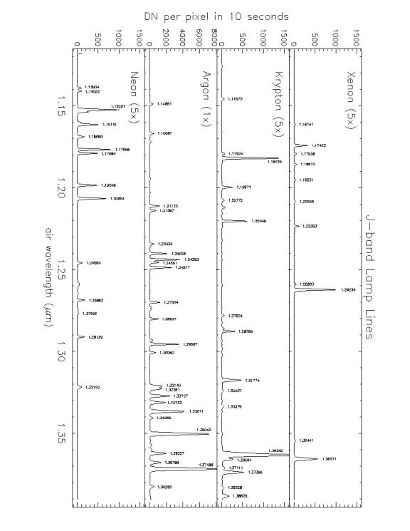 Figure
1: J band
Xenon, Krypton, Argon, and Neon arc lamp spectra at a resolving power of ~ 1000.
Figure
1: J band
Xenon, Krypton, Argon, and Neon arc lamp spectra at a resolving power of ~ 1000.
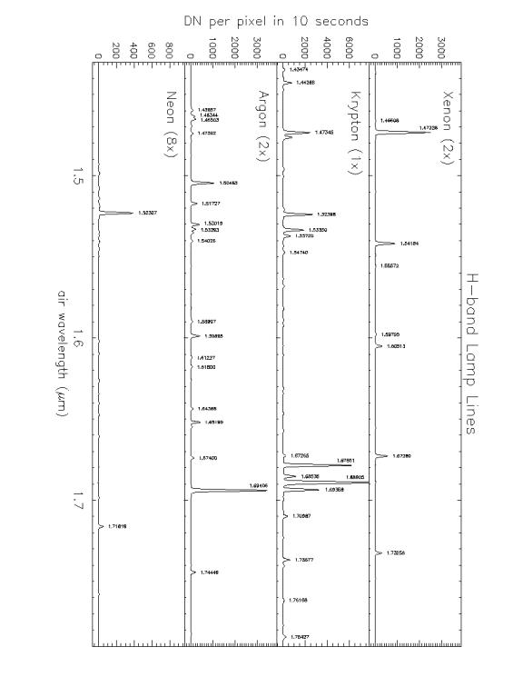
Figure 2: H band Xenon, Krypton, Argon, and Neon arc lamp spectra at a resolving power of ~ 1000.
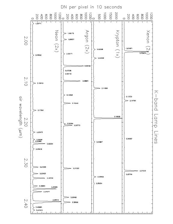
Figure 3: K band Xenon, Krypton, Argon, and Neon arc lamp spectra at a resolving power of ~ 1000.
Appendix H: OH Airglow Wavelengths
Vacuum wavelengths for predominantly OH airglow emission lines are listed in Table 10. Sky spectra are plotted for each NIFS grating below.
Table 10: Vacuum Wavelengths and Relative Intensities of Airglow Emission Lines
|
Wavelength (mm) |
Relative Intensity |
Wavelength (mm) |
Relative Intensity |
|
0.94397 |
5 |
1.14516 |
17 |
|
0.94769 |
5 |
1.15055 |
3 |
|
0.95029 |
4 |
1.15356 |
45 |
|
0.95674 |
4 |
1.15621 |
3 |
|
0.96823 |
4 |
1.15885 |
54 |
|
0.96993 |
4 |
1.116247 |
11 |
|
0.97198 |
4 |
1.16476 |
38 |
|
0.97911 |
7 |
1.16932 |
6 |
|
0.98721 |
11 |
1.17129 |
92 |
|
0.99147 |
12 |
1.17676 |
2 |
|
0.99465 |
21 |
1.17848 |
7 |
|
0.99566 |
18 |
1.18482 |
1 |
|
1.00128 |
22 |
1.18633 |
3 |
|
1.00825 |
14 |
1.19726 |
25 |
|
1.01240 |
17 |
1.19800 |
2 |
|
1.01721 |
22 |
1.19854 |
30 |
|
1.01897 |
16 |
1.19969 |
11 |
|
1.02111 |
21 |
1.20038 |
44 |
|
1.02258 |
12 |
1.20210 |
25 |
|
1.02866 |
39 |
1.20276 |
85 |
|
1.03729 |
26 |
1.20526 |
26 |
|
1.04184 |
29 |
1.21201 |
111 |
|
1.04690 |
22 |
121331 |
40 |
|
1.05248 |
16 |
1.21528 |
18 |
|
1.05859 |
11 |
1.21931 |
38 |
|
1.06523 |
11 |
1.22259 |
109 |
|
1.07288 |
12 |
1.22544 |
59 |
|
1.07432 |
4 |
1.22836 |
113 |
|
1.07510 |
49 |
1.23225 |
22 |
|
1.07721 |
16 |
1.23482 |
82 |
|
1.08313 |
60 |
1.23975 |
6 |
|
1.08418 |
22 |
1.24199 |
114 |
|
1.08957 |
11 |
1.24793 |
3 |
|
1.09234 |
27 |
1.24990 |
31 |
|
1.09484 |
11 |
1.25855 |
4 |
|
1.09723 |
39 |
1.26857 |
80 |
|
1.10063 |
11 |
1.26951 |
64 |
|
1.10268 |
28 |
1.27020 |
37 |
|
1.10694 |
8 |
1.27140 |
39 |
|
1.10870 |
17 |
1.27261 |
20 |
|
1.11379 |
1 |
1.27446 |
24 |
|
1.11530 |
4 |
1.27493 |
45 |
|
1.13098 |
3 |
1.27609 |
76 |
|
1.13281 |
6 |
1.27760 |
32 |
|
1.13511 |
3 |
1.27791 |
149 |
|
1.14398 |
22 |
1.27980 |
57 |
|
1.28035 |
107 |
1.56982 |
41 |
|
1.28248 |
25 |
1.57560 |
8 |
|
1.28311 |
58 |
1.58000 |
5 |
|
1.28450 |
35 |
1.58291 |
338 |
|
1.28660 |
31 |
1.58441 |
92 |
|
1.29019 |
261 |
1.58656 |
29 |
|
1.29178 |
84 |
1.58943 |
5 |
|
1.29399 |
26 |
1.59682 |
100 |
|
1.29821 |
67 |
1.60264 |
299 |
|
1.30181 |
187 |
1.60754 |
125 |
|
1.30492 |
82 |
1.61242 |
296 |
|
1.30817 |
277 |
1.61902 |
61 |
|
1.31242 |
99 |
1.62309 |
297 |
|
1.31532 |
77 |
1.62659 |
36 |
|
1.32072 |
47 |
1.62753 |
1 |
|
1.32329 |
104 |
1.62978 |
14 |
|
1.33210 |
29 |
1.63111 |
5 |
|
1.34179 |
26 |
1.63127 |
72 |
|
1.44652 |
7 |
1.63373 |
56 |
|
1.45150 |
22 |
1.63468 |
138 |
|
1.45600 |
12 |
1.63559 |
24 |
|
1.46008 |
19 |
1.63840 |
51 |
|
1.46611 |
5 |
1.64102 |
16 |
|
1.46944 |
15 |
1.64377 |
174 |
|
1.47360 |
6 |
1.64431 |
19 |
|
1.47797 |
13 |
1.64720 |
20 |
|
1.47958 |
2 |
1.64746 |
63 |
|
1.48017 |
13 |
1.64979 |
152 |
|
1.48290 |
22 |
1.65493 |
92 |
|
1.48603 |
6 |
1.65818 |
3 |
|
1.48836 |
30 |
1.66065 |
20 |
|
1.49050 |
4 |
1.66879 |
431 |
|
1.49278 |
9 |
1.67045 |
144 |
|
1.50523 |
102 |
1.67282 |
46 |
|
1.50651 |
38 |
1.67590 |
6 |
|
1.50841 |
11 |
1.68359 |
71 |
|
1.51830 |
20 |
1.68991 |
244 |
|
1.52368 |
90 |
1.69504 |
122 |
|
1.52836 |
45 |
1.70041 |
301 |
|
1.53282 |
177 |
1.70737 |
82 |
|
1.53911 |
54 |
1.71190 |
199 |
|
1.54279 |
163 |
1.72056 |
60 |
|
1.54579 |
4 |
1.72439 |
107 |
|
1.54966 |
17 |
1.72781 |
47 |
|
1.55055 |
44 |
1.72986 |
12 |
|
1.55136 |
20 |
1.73261 |
58 |
|
1.55361 |
71 |
1.73464 |
53 |
|
1.55419 |
44 |
1.73549 |
42 |
|
1.55659 |
32 |
1.73791 |
60 |
|
1.55934 |
113 |
1.73819 |
126 |
|
1.56271 |
… |
1.74223 |
45 |
|
1.56273 |
56 |
1.74452 |
160 |
|
1.56507 |
188 |
1.74964 |
9 |
|
1.56527 |
… |
1.75011 |
55 |
|
1.75246 |
28 |
2.22381: |
54 |
|
1.76483 |
363 |
2.22978: |
104 |
|
1.76673 |
130 |
2.24381: |
31 |
|
1.76933 |
52 |
2.24948: |
53 |
|
1.77280 |
3 |
2.26620: |
14 |
|
1.78066 |
72 |
2.27097: |
24 |
|
1.78754 |
268 |
|
|
|
1.79316: |
95 |
|
|
|
1.79890 |
204 |
|
|
|
1.80630 |
84 |
|
|
|
1.81135 |
27 |
|
|
|
1.95233 |
14 |
|
|
|
1.95557 |
10 |
|
|
|
1.95881 |
6 |
|
|
|
1.96371 |
18 |
|
|
|
1.96726 |
7 |
|
|
|
1.96967 |
32 |
|
|
|
1.97461 |
10 |
|
|
|
1.97665 |
46 |
|
|
|
1.98343 |
15 |
|
|
|
2.00025 |
93 |
|
|
|
2.00260 |
28 |
|
|
|
2.00622 |
5 |
|
|
|
2.01929: |
93 |
|
|
|
2.02709: |
243 |
|
|
|
2.03370: |
122 |
|
|
|
2.04060: |
281 |
|
|
|
2.04961: |
106 |
|
|
|
2.05561: |
216 |
|
|
|
2.06672: |
68 |
|
|
|
2.07153: |
129 |
|
|
|
2.08504: |
38 |
|
|
|
2.08924: |
70 |
|
|
|
2.09494: |
18 |
|
|
|
2.09704: |
35 |
|
|
|
2.09975 |
72 |
|
|
|
2.10425 |
112 |
|
|
|
2.10785 |
28 |
|
|
|
2.10995: |
147 |
|
|
|
2.11446 |
18 |
|
|
|
2.11656 |
157 |
|
|
|
2.12256: |
33 |
|
|
|
2.12376: |
131 |
|
|
|
2.13247: |
17 |
|
|
|
2.14988: |
223 |
|
|
|
2.15108: |
115 |
|
|
|
2.15349: |
56 |
|
|
|
2.17150: |
62 |
|
|
|
2.17930: |
165 |
|
|
|
2.18711: |
81 |
|
|
|
2.19492: |
200 |
|
|
|
2.20452: |
79 |
|
|
|
2.21157: |
156 |
|
|
Appendix I: Terrestrial Atmospheric Absorption
This section will contain plots of the transmission of the Earth’s atmosphere in the 0.94-2.50 mm range.
Appendix J: List of Figures
|
Figure 1 |
figure.gif |
|
|
|